ggplot(data = ehs_tidy) +
  geom_histogram(aes(x = gross_income))
Choose an appropriate visualisation to check the distribution of the gross income variable from respondents of the English Housing survey. Comment on your findings.
The most appropriate visualisation to check the distribution of a numeric variable is a histogram. This can be created using the geom_histogram function within ggplot2:
ggplot(data = ehs_tidy) +
geom_histogram(aes(x = gross_income))
The histogram shows a strange peak at £100,000. This is because a value of 100000 in this data actually represents any household with a gross income of £100,000 or more. To avoid this distorting our visualisation and any future analysis, we will remove any observations with this value and save it as a new dataset:
ehs_tidy_new <- filter(ehs_tidy,
gross_income != 100000)Removing these observations means losing all of the information recorded on these respondents. We always want to keep the data in its fullest form where possible. Where we need a categorical versions of this variable, this can be included within the same dataset but always keep the raw data.
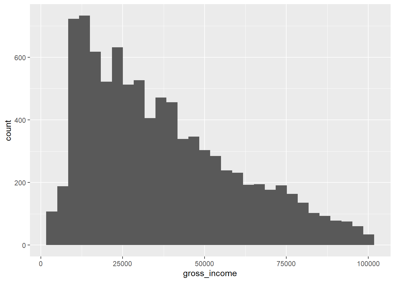
ggplot(data = ehs_tidy_new) +
  geom_histogram(aes(x = gross_income))
The gross income of respondents (that earned less than £100,000) is not normally distributed. The upper tail is longer than the lower tail, making this variable positively/upwardly/right skewed.
Based on the output from question 1, generate a summary table giving the minimum, maximum gross income, and an appropriate measure of the centre and spread of this variable.
In question 1, we saw that the variable was not normally distributed, making the mean and standard deviation inappropriate summary measures. As an alternative, we will display the median as a measure of centre, and the interquartile range (IQR) as a measure of spread.
To create a summary table, use the summarise function. Be sure to use the data without the categorised income to avoid invalid results:
summarise(ehs_tidy_new,
  min_income = min(gross_income),
  max_income = max(gross_income),
  median_income = median(gross_income),
  iqr_income = IQR(gross_income))
# A tibble: 1 × 4
min_income max_income median_income iqr_income
<dbl> <dbl> <dbl> <dbl>
1 3088. 99900. 31768. 33282.